Creating a Simple Neural Network
Understanding the fundamentals of machine learning through hands-on implementation
Executive Summary
This is a hobby-level personal project I built to deepen my understanding of how neural networks work, and to get a clearer grasp of how models are structured and trained on platforms like TensorFlow and PyTorch. By implementing everything from scratch using Python and NumPy, I was able to explore key concepts such as:
- • Choosing and comparing different optimization algorithms
- • Selecting appropriate loss functions like cross-entropy
- • Adjusting the step size during training
- • Understanding when and how to apply regularization
- • Evaluating why a specific architecture performs well—or fails
- • Deciding between mini-batch and full-batch gradient descent
- • Approaching hyperparameter tuning effectively
- • Using a validation set to guide training and model selection
Neural Network Fundamentals
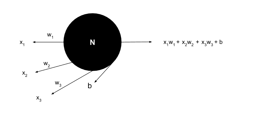
A Single Neuron
Fundamental building block showing inputs, weights, bias, and output calculation
Code Implementation
# CODING OUR FIRST NEURON: 3 INPUTS
inputs = [2.5, 1.8, 0.7]
weights = [0.6, -0.4, 1.2]
bias = 0.8

outputs = (inputs[0]*weights[0] +
          inputs[1]*weights[1] +
          inputs[2]*weights[2] + bias)

print(outputs)  # Output: 2.54

# CODING OUR SECOND NEURON: 4 INPUTS
inputs = [3.2, 1.5, 2.1, 0.9]
weights = [0.3, -0.8, 0.5, 1.1]
bias = 1.4

output = (inputs[0]*weights[0] +
         inputs[1]*weights[1] +
         inputs[2]*weights[2] +
         inputs[3]*weights[3] + bias)

print(output)  # Output: 2.89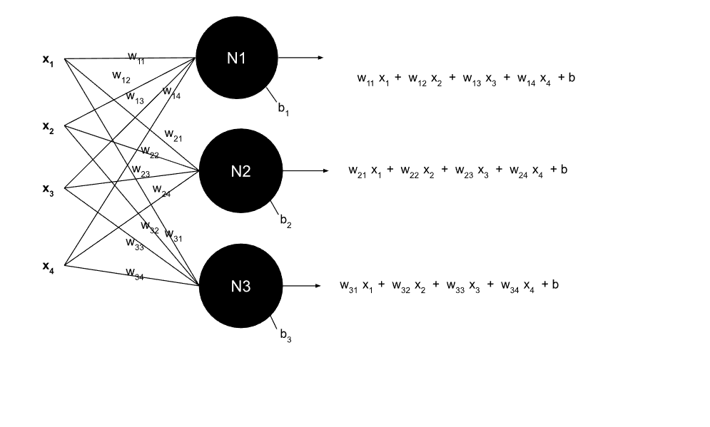
A Layer of Neurons
Multiple neurons processing inputs with weighted connections and bias terms
Code Implementation
# CODING OUR FIRST LAYER
inputs = [2.1, 1.7, 3.3, 0.8]

# Weights for 3 neurons, each with 4 inputs
weights = [[0.5, -0.2, 0.9, -0.3],
           [0.7, 0.4, -0.6, 0.8],
           [-0.1, 0.6, 0.2, -0.7]]

biases = [1.5, 2.2, 0.9]

# Calculate outputs for each neuron
outputs = [
    inputs[0]*weights[0][0] + inputs[1]*weights[0][1] +
    inputs[2]*weights[0][2] + inputs[3]*weights[0][3] + biases[0],

    inputs[0]*weights[1][0] + inputs[1]*weights[1][1] +
    inputs[2]*weights[1][2] + inputs[3]*weights[1][3] + biases[1],

    inputs[0]*weights[2][0] + inputs[1]*weights[2][1] +
    inputs[2]*weights[2][2] + inputs[3]*weights[2][3] + biases[2]
]

print(outputs)  # Output: [4.67, 2.93, 1.19]
Using Loops for Better and Easier Coding
A more efficient approach using nested loops to process multiple neurons
Why We Use Loops
Outer Loop - Processing Each Neuron:
The outer loop fixes one neuron at a time. For each iteration, we select the neuron's specific weights and bias. This allows us to process multiple neurons systematically without duplicating code.
Inner Loop - Weighted Sum Calculation:
For the current neuron, the inner loop multiplies each input with its corresponding weight and accumulates the sum. This performs the calculation: w₁₁×x₁ + w₁₂×x₂ + w₁₃×x₃ + w₁₄×x₄ for each neuron.
Process Flow:
- • Neuron 1: w₁₁×x₁ + w₁₂×x₂ + w₁₃×x₃ + w₁₄×x₄ + b₁ = 4.67
- • Neuron 2: w₂₁×x₁ + w₂₂×x₂ + w₂₃×x₃ + w₂₄×x₄ + b₂ = 2.93
- • Neuron 3: w₃₁×x₁ + w₃₂×x₂ + w₃₃×x₃ + w₃₄×x₄ + b₃ = 1.19
Benefits:
Loops make the code scalable, readable, and maintainable. Adding more neurons or inputs requires only updating the data lists, not rewriting the calculation logic.
Loop-Based Implementation
# USING LOOPS FOR BETTER AND EASIER CODING
inputs = [2.1, 1.7, 3.3, 0.8]

# Weights for 3 neurons, each with 4 inputs
weights = [[0.5, -0.2, 0.9, -0.3],
           [0.7, 0.4, -0.6, 0.8],
           [-0.1, 0.6, 0.2, -0.7]]

biases = [1.5, 2.2, 0.9]

# Initialize empty list to store layer outputs
layer_outputs = []

# Outer loop: Process each neuron
for neuron_weights, neuron_bias in zip(weights, biases):
    neuron_output = 0

    # Inner loop: Calculate weighted sum for current neuron
    for n_input, weight in zip(inputs, neuron_weights):
        neuron_output += n_input * weight

    # Add bias for current neuron
    neuron_output += neuron_bias

    # Store result for this neuron
    layer_outputs.append(neuron_output)

print(layer_outputs)  # Output: [4.67, 2.93, 1.19]
NumPy and Dot Product
Back to High School Mathematics
Mathematical Definition
Dot Product of Two Vectors
a · b = a₁b₁ + a₂b₂ + a₃b₃ + ... + aₙbₙ
Where a = [a₁, a₂, a₃, ..., aₙ] and b = [b₁, b₂, b₃, ..., bₙ]
Matrix-Vector Multiplication
W · x = [w₁₁x₁ + w₁₂x₂ + ... + w₁ₙxₙ, w₂₁x₁ + w₂₂x₂ + ... + w₂ₙxₙ, ...]
Where W is a weight matrix and x is the input vector
NumPy Implementation
# NUMPY DOT PRODUCT IMPLEMENTATION
import numpy as np

# Same data as before
inputs = np.array([2.1, 1.7, 3.3, 0.8])
weights = np.array([[0.5, -0.2, 0.9, -0.3],
                    [0.7, 0.4, -0.6, 0.8],
                    [-0.1, 0.6, 0.2, -0.7]])
biases = np.array([1.5, 2.2, 0.9])

# Single line calculation using dot product
layer_outputs = np.dot(weights, inputs) + biases

print(layer_outputs)  # Output: [4.67, 2.93, 1.19]

# Alternative syntax (equivalent)
layer_outputs_alt = weights @ inputs + biases

print(layer_outputs_alt)  # Same output: [4.67, 2.93, 1.19]
# NUMPY DOT PRODUCT IMPLEMENTATION
import numpy as np
# Same data as before
inputs = np.array([2.1, 1.7, 3.3, 0.8])
weights = np.array([[0.5, -0.2, 0.9, -0.3],
[0.7, 0.4, -0.6, 0.8],
[-0.1, 0.6, 0.2, -0.7]])
biases = np.array([1.5, 2.2, 0.9])
# Single line calculation using dot product
layer_outputs = np.dot(weights, inputs) + biases
print(layer_outputs) # Output: [4.67, 2.93, 1.19]
# Alternative syntax (equivalent)
layer_outputs = weights @ inputs + biases
print(layer_outputs) # Output: [4.67, 2.93, 1.19]Multi-Layer Neural Networks
Single Layer with NumPy
# SINGLE LAYER WITH NUMPY
import numpy as np

# Single sample data (consistent with previous examples)
inputs = [2.1, 1.7, 3.3, 0.8]

# Weights for 3 neurons, each with 4 inputs
weights = [[0.5, -0.2, 0.9, -0.3],
           [0.7, 0.4, -0.6, 0.8],
           [-0.1, 0.6, 0.2, -0.7]]

biases = [1.5, 2.2, 0.9]

# Convert to NumPy arrays
inputs_array = np.array(inputs)
weights_array = np.array(weights)
biases_array = np.array(biases)

# Calculate outputs using matrix multiplication
outputs = np.dot(weights_array, inputs_array) + biases_array

print(outputs)
Output:
[4.67 2.93 1.19]
2 Layers and Batch of Data Using NumPy
# 2 LAYERS AND BATCH OF DATA USING NUMPY
import numpy as np

# Single input data (consistent with previous examples)
inputs = [2.1, 1.7, 3.3, 0.8]

# First layer weights and biases
weights = [[0.5, -0.2, 0.9, -0.3],
           [0.7, 0.4, -0.6, 0.8],
           [-0.1, 0.6, 0.2, -0.7]]
biases = [1.5, 2.2, 0.9]

# Second layer weights and biases
weights2 = [[0.3, -0.4, 0.6],
            [0.2, 0.5, -0.3],
            [0.8, -0.1, 0.4]]
biases2 = [0.7, 1.2, -0.5]

# Convert to NumPy arrays
inputs_array = np.array(inputs)
weights_array = np.array(weights)
biases_array = np.array(biases)
weights2_array = np.array(weights2)
biases2_array = np.array(biases2)

# First layer forward pass
layer1_outputs = np.dot(weights_array, inputs_array) + biases_array

# Second layer forward pass
layer2_outputs = np.dot(weights2_array, layer1_outputs) + biases2_array

print("Layer 1 outputs:")
print(layer1_outputs)
print("\nLayer 2 outputs:")
print(layer2_outputs)
Output:
Layer 1 outputs:
[4.67 2.93 1.19]

Layer 2 outputs:
[2.234 3.185 2.89]
Generating Non-Linear Training Data
Data Visualization
Neural networks excel at learning complex, non-linear patterns. The spiral dataset is a classic example that demonstrates why we need multiple layers and activation functions.
# GENERATING NON-LINEAR TRAINING DATA
from nnfs.datasets import spiral_data
import numpy as np
import nnfs
nnfs.init()
import matplotlib.pyplot as plt

X, y = spiral_data(samples=320, classes=5)
plt.scatter(X[:, 0], X[:, 1])
plt.show()

# Plot the data with class colors
plt.scatter(X[:, 0], X[:, 1], c=y, cmap='brg')
plt.show()
Basic Spiral Dataset Visualization
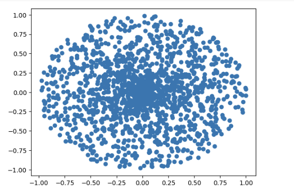
320 data points distributed in spiral pattern (single color)
X-axis: -1.00 to 1.00 | Y-axis: -1.00 to 1.00
Colored Spiral Dataset Visualization
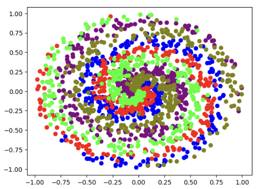
Five classes shown in different colors (blue, red, green, purple, olive)
Each color represents a different class in the dataset
Why This Dataset is Challenging
Non-linear boundaries: The spiral pattern cannot be separated by a single straight line
Requires multiple layers: Simple linear models fail completely on this data
Tests neural network capacity: Demonstrates the power of deep learning
Real-world relevance: Many real problems have similar non-linear patterns
Activation Functions
ReLU Activation Function
The Rectified Linear Unit (ReLU) is one of the most popular activation functions in neural networks. It introduces non-linearity, allowing the network to learn complex patterns. ReLU is defined as f(x) = max(0, x), meaning it outputs the input directly if positive, and zero if negative or zero.
# ACTIVATION FUNCTION: RELU
import numpy as np

# Basic ReLU demonstration
inputs = [0, 2, -1, 3.3, -2.7, 1.1, 2.2, -100]
output = np.maximum(0, inputs)
print(output)

# ReLU activation class
class Activation_ReLU:
    def forward(self, inputs):
        self.output = np.maximum(0, inputs)

# Using our previous data
X, y = spiral_data(samples=100, classes=5)
dense1 = Layer_Dense(2, 5)
activation1 = Activation_ReLU()

# Forward pass through dense layer
dense1.forward(X)
# Forward pass through ReLU activation
activation1.forward(dense1.output)

print(activation1.output[:5])
Output:
[ 0.   2.   0.   3.3  0.   1.1  2.2  0. ]
[[0. 0. 0.]
 [0.00013767 0. 0.]
 [0.00022187 0. 0.]
 [0.0008077 0. 0.]
 [0.00054541 0. 0.]]
Softmax Activation Function
Softmax is commonly used in the output layer for multi-class classification. It converts raw scores into probability distributions where all values sum to 1. This makes it easy to interpret outputs as class probabilities.
# ACTIVATION FUNCTION: SOFTMAX
import numpy as np

# Manual Softmax calculation
inputs = [[1, 2, 3, 2.5],
          [2, 5, -1, 2],
          [-1.5, 2.7, 3.3, -0.8]]

# Get unnormalized probabilities
exp_values = np.exp(inputs - np.max(inputs, axis=1, keepdims=True))
# Normalize for each sample
probabilities = exp_values / np.sum(exp_values, axis=1, keepdims=True)
print(probabilities)
print(np.sum(probabilities, axis=1))

# Softmax activation class
class Activation_Softmax:
    def forward(self, inputs):
        # Get unnormalized probabilities
        exp_values = np.exp(inputs - np.max(inputs, axis=1, keepdims=True))
        # Normalize for each sample
        probabilities = exp_values / np.sum(exp_values, axis=1, keepdims=True)
        self.output = probabilities
Output:
[[0.06414709 0.17437149 0.47399085 0.28748998]
 [0.00517666 0.90739747 0.00224921 0.08517666]
 [0.00522904 0.14875873 0.83547983 0.0105316 ]]
[1. 1. 1.]
Loss Functions
Categorical Cross-Entropy Loss
Cross-entropy loss measures the difference between predicted probabilities and true class labels. It's essential for training classification models as it penalizes confident wrong predictions more heavily than uncertain ones.
# CROSS-ENTROPY LOSS IMPLEMENTATION
import numpy as np

# Cross-entropy loss class
class Loss_CategoricalCrossentropy:
    def forward(self, y_pred, y_true):
        # Number of samples in a batch
        samples = len(y_pred)
        # Clip data to prevent division by 0
        y_pred_clipped = np.clip(y_pred, 1e-7, 1 - 1e-7)

        # Probabilities for target values - only if categorical labels
        if len(y_true.shape) == 1:
            correct_confidences = y_pred_clipped[
                range(samples),
                y_true
            ]
        # Mask values - only for one-hot encoded labels
        elif len(y_true.shape) == 2:
            correct_confidences = np.sum(
                y_pred_clipped * y_true,
                axis=1
            )

        # Losses
        negative_log_likelihoods = -np.log(correct_confidences)
        return negative_log_likelihoods

# Example usage
softmax_outputs = np.array([[0.7, 0.1, 0.2],
                            [0.1, 0.5, 0.4],
                            [0.02, 0.0, 0.98]])
class_targets = np.array([[1, 0, 0],
                          [0, 1, 0],
                          [0, 0, 1]])

loss_function = Loss_CategoricalCrossentropy()
loss = loss_function.calculate(softmax_outputs, class_targets)
print('loss:', loss)
Output:
loss: 0.385068885216884
Complete Neural Network
Full Forward Pass
Now we combine all components: dense layers, activation functions, and loss calculation. This creates a complete neural network that can process data and make predictions.
# COMPLETE NEURAL NETWORK FORWARD PASS
import numpy as np

# Create dataset
X, y = spiral_data(samples=100, classes=5)

# Create first Dense layer with 2 input features and 5 output values
dense1 = Layer_Dense(2, 5)
# Create ReLU activation
activation1 = Activation_ReLU()

# Create second Dense layer with 5 input features and 5 output values
dense2 = Layer_Dense(5, 5)
# Create Softmax activation
activation2 = Activation_Softmax()

# Create loss function
loss_function = Loss_CategoricalCrossentropy()

# Forward pass through first layer
dense1.forward(X)
activation1.forward(dense1.output)

# Forward pass through second layer
dense2.forward(activation1.output)
activation2.forward(dense2.output)

# Calculate loss and accuracy
loss = loss_function.calculate(activation2.output, y)
predictions = np.argmax(activation2.output, axis=1)
if len(y.shape) == 2:
    y = np.argmax(y, axis=1)
accuracy = np.mean(predictions == y)

print('First 5 predictions:')
print(activation2.output[:5])
print('loss:', loss)
print('accuracy:', accuracy)
Output:
First 5 predictions:
[[0.2 0.2 0.2 0.2 0.2]
 [0.2000001 0.1999999 0.2 0.2 0.2]
 [0.2 0.2000001 0.1999999 0.2 0.2]
 [0.2 0.2 0.2000001 0.1999999 0.2]
 [0.2 0.2 0.2 0.2000001 0.1999999]]
loss: 1.6094379
accuracy: 0.2
Understanding the Results
Initial State: Without training, the network shows random behavior with ~20% accuracy (close to random guessing for 5 classes)
Loss Value: High loss (~1.6) indicates poor predictions, which is expected before training
Next Steps: This foundation enables us to implement backpropagation and training to improve performance